One DBAC step

A DBAC step is one round of cooling: it takes the current state of the data qubit and returns a colder one. In the code it is called a DB-QITE step (double-bracket quantum imaginary-time evolution), and lives in dbac.dbqite. This page shows how to run one, what it computes, and how its two parameters, the duration \(s\) and the number of DME steps \(M\), change the result.

What a step computes

Imaginary-time evolution \(e^{-\tau\hat H}|\psi\rangle\) (normalized) drives any state towards the ground state, but it is not unitary. DBAC approximates a short stretch of it with the double-bracket step

\[ |\psi_\mathrm{DBAC}\rangle = e^{is\hat H}\, e^{is|\psi\rangle\langle\psi|}\, e^{-is\hat H}\,|\psi\rangle . \]

Moving the outer rotations inside the exponential gives an equivalent form that is easier to implement:

\[ |\psi_\mathrm{DBAC}\rangle = e^{is\rho'}\,|\psi\rangle, \qquad \rho' = e^{is\hat H}\,|\psi\rangle\langle\psi|\,e^{-is\hat H}. \]

That is exactly what the code does:

1. rotate a copy of the state about \(\hat H\) to get the instruction \(\rho'\) (on hardware, the \(R_Z(\pi/4)\) gates on the instruction qubits);

2. apply \(e^{is\rho'}\) to the data qubit with DME, using \(M\) copies of \(\rho'\).

Running a step

QITE_dme_select_M(M) returns a step function with the number of DME steps fixed. Call it with a state and a duration \(s\):

import numpy as np
from dbac.dbqite import QITE_dme_select_M, H
from dbac.utils import rx_sweep, fidelity_with_0

def energy(rho):
    """Energy Tr(rho H) of a density matrix."""
    return round(np.trace(rho @ H).real, 6) + 0.0   # + 0.0 turns -0.0 into 0.0

psi = rx_sweep([0.5])[0]                 # theta = pi/4, halfway between |0> and |1>
step = QITE_dme_select_M(1)              # one DME step, like circuit A in the paper

rho = step(psi, np.pi / 4)               # s = pi/4

print(f"before: E = {energy(psi @ psi.conj().T):+.3f}, F = {fidelity_with_0(psi):.3f}")
print(f"after:  E = {energy(rho):+.3f}, F = {fidelity_with_0(rho):.3f}")

before: E = +0.000, F = 0.500
after:  E = -0.500, F = 0.750

The energy dropped from \(0\) to \(-0.5\): the qubit got colder.

The step functions

All step functions share the signature step(psi, s) -> density matrix, so they can be swapped freely, and all of them can be handed to GCI to run several steps.

function	what it does
QITE_dme_select_M(M)	returns a step that uses \(M\) Trotterized DME steps (the realistic, hardware-like case)
ideal_DME	the same step with \(e^{is\rho'}\) applied exactly, i.e. the limit \(M\to\infty\)
initial_psi	does nothing and returns the input; a baseline for “no cooling”
QITE_GCI_dme	the Trotterized step with a default of \(M = 100\)

More DME steps approach the ideal step:

from dbac.dbqite import ideal_DME

for M in (1, 2, 5, 20):
    print(f"M = {M:2d}:      E = {energy(QITE_dme_select_M(M)(psi, np.pi / 4)):+.4f}")
print(f"ideal (M=inf): E = {energy(ideal_DME(psi, np.pi / 4)):+.4f}")

M =  1:      E = -0.5000
M =  2:      E = -0.6036
M =  5:      E = -0.6646
M = 20:      E = -0.6963
ideal (M=inf): E = -0.7071

For the ideal step, the paper gives the energy after one step in closed form (its Eq. 3). With \(E_0\) the energy before the step,

\[ E_\mathrm{DBAC} = E_0 - 2\sin^2(s)\,(1-E_0^2)\,\big[(1-\cos s)\,E_0 + \cos s\big]. \]

E0, s = 0.0, np.pi / 4
print(E0 - 2 * np.sin(s)**2 * (1 - E0**2) * ((1 - np.cos(s)) * E0 + np.cos(s)))

-0.7071067811865475

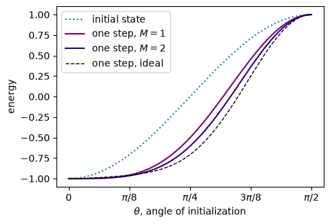
Cooling across all initial states

The same step cools every state except the two poles. \(|0\rangle\) is already cold, and \(|1\rangle\) is an excited eigenstate of \(\hat H\) that imaginary-time evolution cannot move; the factor \((1-E_0^2)\) in the formula above vanishes at both.

import matplotlib.pyplot as plt

fractions = np.linspace(0, 1, 60)
theta = fractions * np.pi / 2
psis = rx_sweep(fractions)

fig, ax = plt.subplots(figsize=(5, 3.4))
ax.plot(theta, [(p.conj().T @ H @ p).item().real for p in psis], ":", label="initial state")
for M, color in [(1, "#7a0085"), (2, "#2c0084")]:
    ax.plot(theta, [energy(QITE_dme_select_M(M)(p, np.pi / 4)) for p in psis],
            color=color, label=f"one step, $M={M}$")
ax.plot(theta, [energy(ideal_DME(p, np.pi / 4)) for p in psis], "k--", lw=1, label="one step, ideal")
ax.set_xticks([0, np.pi / 8, np.pi / 4, 3 * np.pi / 8, np.pi / 2],
              ["0", r"$\pi/8$", r"$\pi/4$", r"$3\pi/8$", r"$\pi/2$"])
ax.set_xlabel(r"$\theta$, angle of initialization")
ax.set_ylabel("energy")
ax.legend();

Choosing the duration \(s\)

The duration \(s\) is a free parameter, and the best value depends on the state and on \(M\). Scanning it for one state shows a clear optimum:

s_values = np.linspace(0, np.pi / 2, 100)

fig, ax = plt.subplots(figsize=(5, 3.2))
for M, color in [(1, "#7a0085"), (2, "#2c0084")]:
    ax.plot(s_values, [energy(QITE_dme_select_M(M)(psi, s)) for s in s_values],
            color=color, label=f"$M={M}$")
ax.axvline(np.pi / 4, color="k", ls=":", lw=1)
ax.set_xlabel("step duration $s$")
ax.set_ylabel(r"energy after one step ($\theta=\pi/4$)")
ax.legend();

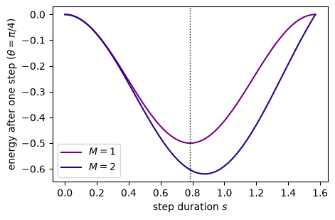
The paper uses \(s = \pi/4\), which cools a wide range of initial states at once. For the recursion, the repository caches optimized durations for every \((M, k)\) in notebooks/optimal_s_Mk.npy: entry [M - 1, j] is the duration of step \(j+1\) when each step uses \(M\) DME steps. scripts/sup_figure_S4.py (load_or_fit_optimal_s_Mk) regenerates it.

optimal_s_Mk = np.load("../../notebooks/optimal_s_Mk.npy")
print("shape (M_max, k_max):", optimal_s_Mk.shape)
print("M = 1, first three steps:", optimal_s_Mk[0, :3].round(3))

shape (M_max, k_max): (10, 7)
M = 1, first three steps: [0.785 0.785 0.785]

Next

One step only cools so far. Running the recursion shows how to chain steps, using each cooled state as the instruction for the next.