Double-Bracket Algorithmic Cooling (DBAC)

Code accompanying Double-Bracket Algorithmic Cooling (M. Alghadeer, K. U. Giang, S. Cao, S. D. Fasciati, M. Piscitelli, N. Ng, P. J. Leek, M. Gluza, M. Bakr). This page walks through the paper’s main experimental result (its Fig. 4): how much a single qubit is cooled by DBAC as we spend more qubits as resources, compared with data taken on a superconducting-qubit device.

The dbac package provides the DME implementations, the DB-QITE/GCI recursion, the HBAC baseline and all the plotting code used for the paper figures. See Installation to set it up, the Quick start for a first example, the guide for how each part works, and the API reference for every function.

Background: cooling a qubit by removing its coherence

Algorithmic cooling (AC) lowers the entropy of one qubit by moving entropy into other qubits using only unitary operations. DBAC solves a complementary problem. The qubits carry no entropy: every one of them is prepared in the same pure state \(|\psi\rangle\), but we do not know which state it is, and we cannot measure it without collapsing the superposition. The goal is still to rotate one qubit to the ground state \(|0\rangle\), that is, to remove its quantum coherence.

Learning \(|\psi\rangle\) first (tomography) does not escape the problem: the statistical error only falls as \(1/\sqrt{n}\) in the number of copies \(n\). DBAC instead uses the other copies of \(|\psi\rangle\) directly as quantum instructions: they act as a temporary Hamiltonian that tells the target qubit which way to rotate, with no measurement and no feedback. The circuit itself is the same for every input state, and the state it meets decides what it does.

As in Nernst’s unattainability principle, perfect cooling would need infinitely many instructions. With a finite number of qubits the cooling is partial, and it improves as more qubits are added. This page shows that trade-off.

How DBAC works

Imaginary-time evolution. Evolving in imaginary time under a Hamiltonian \(\hat H\),

\[ |\psi(\tau)\rangle = \frac{e^{-\tau \hat H}|\psi\rangle}{\lVert e^{-\tau \hat H}|\psi\rangle\rVert}, \]

maps any pure state to another pure state that gets closer to the ground state of \(\hat H\) as \(\tau\) grows, unless the input is an exact excited eigenstate. DBAC uses \(\hat H = -Z\), so the ground state is \(|0\rangle\) with energy \(-1\) and the excited state is \(|1\rangle\) with energy \(+1\). The energy of the data qubit is \(E = \langle\psi|\hat H|\psi\rangle\).

One DBAC step. Imaginary-time evolution is not unitary, but for a single qubit it can be approximated by a double-bracket step built from the group commutator. A reflection about the state itself, \(e^{it|\psi\rangle\langle\psi|}\), is sandwiched between two rotations about \(\hat H\):

\[ |\psi_\mathrm{DBAC}\rangle = e^{it\hat H}\, e^{it|\psi\rangle\langle\psi|}\, e^{-it\hat H}\,|\psi\rangle . \]

When the reflection is applied exactly, the energy after one step with duration \(t\), starting from energy \(E_0\), is known in closed form (Eq. 3 of the paper):

\[ E_\mathrm{DBAC} = E_0 - 2\sin^2(t)\,(1-E_0^2)\,\Big[(1-\cos t)\,E_0 + \cos t\Big]. \]

The correction vanishes for \(E_0=\pm1\). The two poles \(|0\rangle\) and \(|1\rangle\) are therefore fixed points: \(|0\rangle\) is already cold, and \(|1\rangle\) is an excited eigenstate that the flow cannot move. Every other state is cooled.

Density-matrix exponentiation (DME). The reflection \(e^{it|\psi\rangle\langle\psi|}\) would need to know \(|\psi\rangle\). DME avoids this by using a copy of the state as the Hamiltonian. For a small duration \(t\), a partial SWAP between a data qubit \(\sigma\) and an instruction qubit \(\rho\) gives

\[ \mathrm{Tr}_2\!\left[e^{-it\,\mathrm{SWAP}}(\sigma\otimes\rho)\,e^{it\,\mathrm{SWAP}}\right] = \sigma - it[\rho,\sigma] + O(t^2) \approx e^{-it\rho}\,\sigma\, e^{it\rho}. \]

The partial SWAP \(U_\mathrm{DME}(\varphi)=e^{i\varphi\,\mathrm{SWAP}}\) is the same circuit for every \(\rho\), so the information in \(\rho\) decides which rotation is applied. On hardware it is compiled from the Heisenberg interaction \(XX+YY+ZZ\) using the native \(ZZ\) interaction of the transmons (\(U_\mathrm{DME}(\varphi) = R_{ZZ}(\varphi)\,R_{YY}(\varphi)\,R_{XX}(\varphi)\)).

Two knobs: \(M\) and \(k\). Using one copy per DME call only approximates the exponential. Two independent resources then control how well DBAC cools:

symbol	meaning	what it costs
\(M\)	number of DME steps (Trotter steps) inside one DBAC step. The duration \(t\) is split into \(M\) pieces \(t/M\), each using a fresh copy of the instruction state, and the error of the approximation shrinks as \(O(t^2/M)\).	\(M\) copies of $
\(k\)	number of DBAC steps, applied recursively. Step \(k+1\) uses the cooled output of step \(k\) as its instruction, so each step starts from a colder state.	the instructions of step \(k\) must be prepared first, in parallel, so the copies multiply

More of either resource means more qubits \(n\) in the circuit and lower energy of the data qubit.

The experiment

Every circuit is run as follows.

1. Prepare. All \(n\) qubits start in \(|0\rangle\) and receive the same rotation \(R_X(\theta)\), so each holds \(|\psi(\theta)\rangle = R_X(\theta)|0\rangle\). In the paper’s convention \(R_X(\theta)=e^{-i\theta X}\), so \(\theta=0\) is the ground state \(|0\rangle\), the energy rises as \(\theta\) grows, and \(\theta=\pi/2\) is the excited state \(|1\rangle\). The energy of the untouched state is \(E_0(\theta) = -\cos 2\theta\).

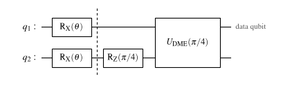
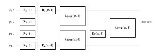
2. Apply DBAC with \(k\) DBAC steps and \(M\) DME steps each. On the instruction qubits, \(R_Z(\pi/4) = e^{-it\hat H}\) with \(t=\pi/4\) prepares \(e^{-it\hat H}|\psi\rangle\). The data qubit then interacts with the instructions through \(U_\mathrm{DME}\). The final rotation \(e^{it\hat H}\) on the data qubit is a \(Z\) rotation and does not change its energy, so it is left out of the hardware circuits.

3. Read out the energy of the data qubit and repeat for a sweep of \(\theta\).

Without DBAC the energy follows the Initial state curve \(-\cos 2\theta\). After DBAC it should move toward the ground-state value \(-1\).

The three circuits below are the ones run on the device. Dashed lines separate the DBAC steps.

circuit	\(k\) (DBAC steps)	\(M\) (DME steps)	qubits \(n\)	instruction copies
A	1	1	2	1
B	1	2	3	2
C	2	1	4	3

The code that generates the circuits’ energy curves, the digitized experimental data and the plot styling is in scripts/figure_4.py, and the plotting code is in src/dbac/plotting/.

%matplotlib inline
import sys
sys.path.append('..')
sys.path.append('../src')
sys.path.append('../notebooks')  # for config.py

import numpy as np

from config import plot_path
from dbac.plotting import use_paper_style, figure_size, plot_single_energy_curve, draw_dbac_circuit
from scripts.figure_4 import (
    CIRCUIT_COLORS, CIRCUIT_FILENAMES, CIRCUIT_MARKERS, EXPERIMENTAL_ENERGY,
    OPTIMAL_S_PATH, XTICKS, XTICK_LABELS, run_dbac_circuits,
)
from dbac.gci import GCI
from dbac.dbqite import initial_psi
from dbac.utils import rx_sweep

use_paper_style(font_size=10, figsize=figure_size("PRD", "onecol"))

[Qibo 0.3.6|INFO|2026-10-26 14:05:21]: Using numpy backend on /CPU:0

Simulating DBAC

For each \(\theta\) we build \(|\psi(\theta)\rangle = R_X(\theta)|0\rangle\) and run DB-QITE with the step durations optimized for each \((M, k)\) (cached in optimal_s_Mk.npy). The result is the analytical curve of each circuit, from noiseless simulation with \(M\)-step Trotterized DME. The Initial state baseline is the energy of \(|\psi(\theta)\rangle\) before any cooling.

optimal_s_Mk = np.load(OPTIMAL_S_PATH)
thetas = np.linspace(0, 1, 100)

psis_energy = rx_sweep(thetas, start=np.array([[1], [0]], dtype=complex))
theta_angles = thetas * np.pi / 2
res_init = [GCI(initial_psi, psi, 1, np.linspace(0.01, 1, 2)).execute_gci()[0][-1] for psi in psis_energy]
energy_results = run_dbac_circuits(psis_energy, optimal_s_Mk, as_fidelity=False)

def plot_circuit_energy(label):
    plot_single_energy_curve(
        theta_angles, res_init, label, energy_results[label],
        CIRCUIT_COLORS[label], CIRCUIT_MARKERS[label],
        experimental=EXPERIMENTAL_ENERGY.get(label),
        xticks=XTICKS, xtick_labels=XTICK_LABELS, show=True,
        save_path=plot_path(CIRCUIT_FILENAMES[label]))

Each circuit individually, overlaid with hardware experiment data

In each plot below, the horizontal axis is the initialization angle \(\theta\) and the vertical axis is the energy of the data qubit after the circuit.

• the dotted curve is the Initial state, the energy \(-\cos 2\theta\) with no cooling;

• the solid curve is the Analytical prediction of DBAC for that circuit;

• the open circles are the Experiment, measured on the superconducting device.

Cooling shows up as a curve below the dotted one, closer to the ground-state energy \(-1\). Both ends are fixed points, as discussed above: \(|0\rangle\langle 0|\) at \(\theta=0\) is already in the ground state, and \(|1\rangle\langle 1|\) at \(\theta=\pi/2\) is an exact excited eigenstate that imaginary-time evolution cannot move.

Circuit A: 1 DBAC step, 1 DME step (\(n=2\))

The minimal DBAC circuit. One instruction qubit is rotated by \(R_Z(\pi/4)\) and the data qubit \(q_1\) is coupled to it through a single \(U_\mathrm{DME}(\pi/4)\). The step duration \(t=\pi/4\) cools a wide range of initial states.

draw_dbac_circuit("A");

plot_circuit_energy(r'$n=2$');

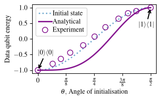
A single instruction already lowers the energy of the data qubit across the sweep. The experimental points lie between the analytical curve and the uncooled baseline: the cooling is real but smaller than in the noiseless simulation, because of gate errors and decoherence. Since \(M=1\), the DME step is also a single, coarse partial SWAP.

Circuit B: 1 DBAC step, 2 DME steps (\(n=3\))

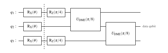
The same total duration \(t=\pi/4\) is now split into \(M=2\) DME steps of \(\pi/8\) each. Each step uses its own instruction copy (\(q_1\) and \(q_3\), both rotated by \(R_Z(\pi/4)\)), and both act on the data qubit \(q_2\). This distributes the DME over two instruction qubits, a finer Trotterization of \(e^{-it\rho}\) than circuit A, at the price of one more qubit.

draw_dbac_circuit("B");

plot_circuit_energy(r'$n=3$');

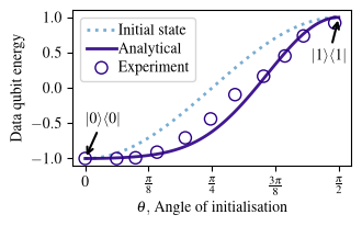
Cooling is stronger than in circuit A: the curve is flatter and sits lower, and the experimental data confirm this. Of the three circuits, this one agrees best with the analytical prediction. The extra instruction qubit improves the DME approximation, which shows that distributing DME improves cooling.

Circuit C: 2 DBAC steps, 1 DME step (\(n=4\))

Here the DBAC recursion is applied twice (\(k=2\)) with a single DME step in each. The first step is circuit A, run twice in parallel: once to cool the data qubit \(q_2\) (instruction \(q_1\)) and once to prepare a cooled copy on \(q_3\) (instruction \(q_4\)). The second step, after the second dashed line, uses that cooled copy on \(q_3\) as the instruction for \(q_2\), so it starts from a colder state than a single step could provide.

draw_dbac_circuit("C");

plot_circuit_energy(r'$n=4$');

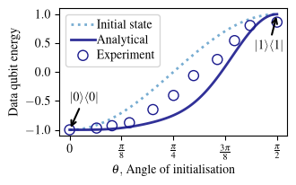
In the noiseless simulation, the two recursion steps cool even more than circuit B. On the device, however, this circuit is the deepest and has the most entangling gates, and the siZZle pulses that implement them are relatively long. Decoherence accumulates, so the experimental points lie well above the analytical curve and only modestly below the uncooled state. Circuit C is at the verge of break-even for this device, even though the analytical curve predicts further cooling with more steps.

Summary

circuit	\(k\)	\(M\)	\(n\)	what it demonstrates
A	1	1	2	the minimal DBAC step: coherence is removed with one instruction and no measurement
B	1	2	3	distributing DME over more instruction qubits improves cooling
C	2	1	4	recursion cools further in theory, but decoherence limits it on today’s device

Starting from \(|\psi(\theta)\rangle = R_X(\theta)|0\rangle\), DBAC with \(k\) DBAC steps and \(M\) DME steps moves the data qubit toward the ground state. Spending more qubits (\(M\) and \(k\)) gives lower energy in theory. Reaching \(|0\rangle\) exactly would take infinitely many instructions, which is the analogue of Nernst’s principle. In practice, hardware noise sets how far the recursion pays off.

To regenerate all figures of the paper, see Reproducing the figures.