Running the recursion

A single DBAC step has a finite cooling limit. To cool further, DBAC is applied recursively: the output of step \(k\) becomes the input, and the instruction, of step \(k+1\). This page shows how to run \(k\) steps with dbac.gci.GCI, how to read its output, and how to measure how much the recursion buys.

The recursion

With \(|\psi_0\rangle = |\psi\rangle\), each step applies

\[ |\psi_{j+1}\rangle = e^{is_{j+1}\hat H}\, e^{is_{j+1}|\psi_j\rangle\langle\psi_j|}\, e^{-is_{j+1}\hat H}\,|\psi_j\rangle, \qquad j = 0, \dots, k-1 . \]

Each step needs copies of the current state as instructions, so those copies must have been cooled by the earlier steps, in parallel. If step \(j\) uses \(M_j\) DME steps, the recursion consumes \(M_1 M_2 \cdots M_k\) copies of the input: the cost grows quickly with \(k\), the resource trade-off that the paper relates to Nernst’s principle.

Running \(k\) steps with GCI

GCI (group commutator iteration) runs any step function repeatedly and records what happens along the way. Give it the step function, the initial state, None, and the list of durations \(s_1, \dots, s_k\):

import numpy as np
from dbac.gci import GCI
from dbac.dbqite import QITE_dme_select_M
from dbac.utils import rx_sweep

psi = rx_sweep([0.6])[0]                       # a fairly hot initial state
s_schedule = [np.pi / 4, np.pi / 4, np.pi / 4]  # k = 3 steps

gci = GCI(QITE_dme_select_M(1), psi, None, s_schedule)
results = gci.execute_gci()

energies, fidelities = np.real(results[0]), results[-1]
for j, (E, F) in enumerate(zip(energies, fidelities)):
    print(f"after {j} steps:  E = {E:+.3f}   F = {F:.3f}")

after 0 steps:  E = +0.309   F = 0.345
after 1 steps:  E = -0.143   F = 0.572
after 2 steps:  E = -0.531   F = 0.765
after 3 steps:  E = -0.673   F = 0.836

Every step lowers the energy, with diminishing returns.

Reading the output

execute_gci() returns a tuple with one entry per quantity. Each list has \(k+1\) entries: the initial state first, then one per step.

index	name	contents
0	energies	energy \(\mathrm{Tr}(\rho\hat H)\) after each step (may be complex-typed; take np.real)
1	step sizes	the durations used, starting with 0 for the initial state
2	variances	energy variance \(\langle\hat H^2\rangle - \langle\hat H\rangle^2\)
3	durations	cumulative evolution time \(\sum_j s_j^2\), the x-axis of plot_gci_results
4, 5	label, marker	display hints copied from the step function
6, 7	circuit depths, circuits	only for qibo-circuit states, otherwise None
8	states	the state after each step
9	final state	the last entry of states
10	fidelities	fidelity with \(\lvert 0\rangle\) after each step

Tip

Indexing from both ends is the easiest way to pick what you need: results[0] for energies, results[-1] for fidelities, results[-2] for the final state.

Two modes: fixed schedule or line search

The third argument, nmb_steps, switches between two modes.

Fixed schedule (nmb_steps=None), as above: the fourth argument is the list of durations, one per step. This is how the paper’s circuits are simulated, with the durations taken from the cached table optimal_s_Mk.npy.

Greedy line search (nmb_steps=k): the fourth argument is a list of candidate durations. At every step GCI tries all of them and keeps the one that gives the lowest energy.

from dbac.dbqite import ideal_DME

candidates = list(np.linspace(0.05, 1.5, 30))
results = GCI(ideal_DME, psi, 3, candidates).execute_gci()

print("chosen durations:", np.round(results[1][1:], 3))
print("energies:        ", np.real(results[0]).round(3))

chosen durations: [1.1 0.8 0.7]
energies:         [ 0.309 -0.585 -0.937 -0.992]

Note

If the best candidate is the first or last value of the list, GCI emits a warning that the edge of the interval was reached: the true optimum may lie outside your candidates. dbac silences this warning on import; re-enable it with warnings.filterwarnings("default", message=".*edge of interval.*") when tuning candidates.

How much does the recursion buy?

Sweeping the initial state shows how each extra step pulls the curve towards perfect cooling. Here the initial state runs from \(|1\rangle\) (fidelity 0) to \(|0\rangle\) (fidelity 1), and each curve uses the optimized durations for \(M=1\):

import matplotlib.pyplot as plt
from dbac.utils import fidelity_with_0

optimal_s_Mk = np.load("../../notebooks/optimal_s_Mk.npy")
psis = rx_sweep(np.linspace(0, 1, 60), start=np.array([[0], [1]], dtype=complex))
F_initial = [fidelity_with_0(p) for p in psis]

fig, ax = plt.subplots(figsize=(5, 3.4))
ax.plot(F_initial, F_initial, ":", label="initial state")
for k, color in [(1, "#7a0085"), (2, "#2c0084"), (3, "#1a1a8d")]:
    s_k = list(optimal_s_Mk[0, :k])
    F_final = [GCI(QITE_dme_select_M(1), p, None, s_k).execute_gci()[-1][-1] for p in psis]
    ax.plot(F_initial, F_final, color=color, label=f"$k={k}$")
ax.set_xlabel("fidelity of initial state with $|0\\rangle$")
ax.set_ylabel("fidelity after DBAC")
ax.legend();

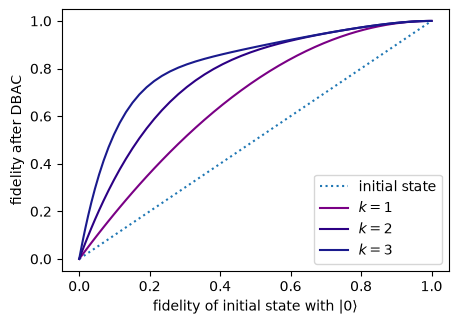
To summarize such a curve with one number, max_excitation finds the initial fidelity at which the final fidelity reaches a target. Anything colder than that is cooled to at least the target:

from dbac.gci import max_excitation

s_2 = list(optimal_s_Mk[0, :2])
F_final = [GCI(QITE_dme_select_M(1), p, None, s_2).execute_gci()[-1][-1] for p in psis]
print("k = 2 reaches F = 0.9 from initial fidelity", round(max_excitation(F_initial, F_final, 0.9), 3))

k = 2 reaches F = 0.9 from initial fidelity 0.566

max_excitation scans the points in order and returns the first one within a tolerance of the target, widening the tolerance until it finds one (or returns None). Pass the sweep from hot to cold, as above, so the first match is the threshold.

Next

DBAC removes coherence. The classic way to cool a qubit removes entropy instead; the HBAC baseline implements it for comparison.