Density matrix exponentiation

Density matrix exponentiation (DME) is the subroutine that lets DBAC work without knowing the state it is cooling. This page explains what it does, how the different implementations in dbac.dme relate to each other, and how the number of Trotter steps \(M\) controls its accuracy.

The problem DME solves

A DBAC step needs to rotate the data qubit \(\sigma\) with the unitary \(e^{it\rho}\), where the “Hamiltonian” \(\rho = |\psi\rangle\langle\psi|\) is the very state we do not know. Compiling \(e^{it\rho}\) as a gate would require tomography of \(|\psi\rangle\) first.

DME avoids this. If we hold a copy of \(\rho\) (the instruction), a short partial SWAP between data and instruction followed by discarding the instruction gives

\[ \mathrm{Tr}_2\!\left[e^{it\,\mathrm{SWAP}}(\sigma\otimes\rho)\,e^{-it\,\mathrm{SWAP}}\right] = \cos^2 t\,\sigma + \sin^2 t\,\rho + i\sin t\cos t\,[\rho,\sigma] \approx e^{it\rho}\,\sigma\,e^{-it\rho}. \]

The SWAP circuit is the same for every \(\rho\). The state of the instruction alone decides which rotation the data qubit receives. This is why the paper calls DBAC a dynamic quantum algorithm, and the copies of \(|\psi\rangle\) quantum instructions.

One DME call

Every implementation takes the data state, the instruction state, the total duration t and the number of Trotter steps M:

import numpy as np
from dbac.dme import dme_channel, dme_expm

def random_pure_state(rng):
    v = rng.normal(size=2) + 1j * rng.normal(size=2)
    v /= np.linalg.norm(v)
    return np.outer(v, v.conj())

rng = np.random.default_rng(1)
data, instruction = random_pure_state(rng), random_pure_state(rng)

exact = dme_expm(data, instruction, t=1.0)            # e^{it rho} sigma e^{-it rho}
approx, history = dme_channel(data, instruction, t=1.0, M=10)

print("distance to exact:", np.linalg.norm(exact - approx))
print("intermediate states returned:", len(history))

distance to exact: 0.12397582390375735
intermediate states returned: 10

dme_channel returns two things: the final data state, and a list with the data state after each of the M steps (useful for plotting convergence).

Trotter steps: spending more copies

Each call to the partial SWAP consumes one instruction copy and is only accurate for a small duration. To reach a finite duration \(t\), DME splits it into \(M\) steps of \(t/M\), each with a fresh copy of \(\rho\):

\[ \left(\hat E^{(\rho)}_{t/M}\right)^{M}(\sigma) = e^{it\rho}\,\sigma\,e^{-it\rho} + O(t^2/M). \]

So \(M\) is a resource knob: \(M\) times more instruction qubits buy an \(M\) times smaller error.

import matplotlib.pyplot as plt

Ms = range(1, 51)
errors = [np.linalg.norm(exact - dme_channel(data, instruction, 1.0, M)[0]) for M in Ms]

fig, ax = plt.subplots(figsize=(5, 3.2))
ax.loglog(Ms, errors, "o", mfc="none", color="#7a0085", label="DME channel")
ax.loglog(Ms, errors[-1] * Ms[-1] / np.array(Ms), "k--", lw=1, label=r"$\propto 1/M$")
ax.set_xlabel("Trotter steps $M$ (instruction copies)")
ax.set_ylabel("distance to exact")
ax.legend();

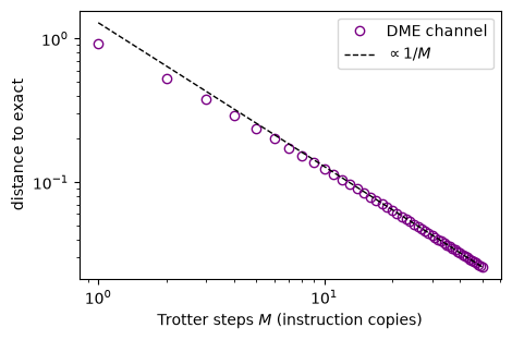
The paper’s hardware circuits use \(M = 1\) and \(M = 2\) (circuits A and B on the front page).

Which implementation should I use?

All of these compute the same channel. They differ in how, and they are kept so that each can be checked against the others (the paper’s Fig. S2, scripts/sup_figure_S2.py).

function	how it computes the channel	use it when
dbac.dme.dme_expm	exact \(e^{it\rho}\sigma e^{-it\rho}\) by matrix exponential (\(M\to\infty\))	you need the ideal reference
dbac.dme.dme_channel	builds \(\sigma\otimes\rho\), applies \(e^{it\,\mathrm{SWAP}/M}\), traces out with numpy	you want the literal two-qubit picture
dbac.dme.dme_qibo	same as above, with qibo’s SWAP gate and partial trace	you want to cross-check against qibo
dbac.dme.dme_channel_equivalent	closed form \(\cos^2\sigma + \sin^2\rho + i\sin\cos[\rho,\sigma]\)	you want speed (no \(4\times 4\) matrices)
dbac.dbqite.DME	the closed form again, returning only the final state	inside DBAC steps (used by QITE_dme_select_M)

from dbac.dme import dme_channel_equivalent, dme_qibo
from dbac.dbqite import DME

M = 5
results = {
    "dme_channel": dme_channel(data, instruction, 1.0, M)[0],
    "dme_channel_equivalent": dme_channel_equivalent(data, instruction, 1.0, M)[0],
    "dme_qibo": dme_qibo(data, instruction, 1.0, M)[0],
    "dbqite.DME": DME(instruction, data, 1.0, M),
}
reference = results["dme_channel"]
for name, rho in results.items():
    print(f"{name:24s} differs from dme_channel by {np.linalg.norm(rho - reference):.1e}")

dme_channel              differs from dme_channel by 0.0e+00
dme_channel_equivalent   differs from dme_channel by 8.3e-16
dme_qibo                 differs from dme_channel by 0.0e+00
dbqite.DME               differs from dme_channel by 8.3e-16

Warning

dbac.dbqite.DME takes its arguments in the order (instruction, data, t, M), the reverse of the functions in dbac.dme, and returns only the final state rather than a (state, history) tuple.

Note

Sign convention. The code implements \(e^{+it\rho}\sigma e^{-it\rho}\) (partial SWAP \(e^{+it\,\mathrm{SWAP}}\)). The paper’s appendix writes the same channel with the opposite sign of \(t\). Both describe the same physics; just keep the sign in mind when comparing formulas.

On hardware

On the device, the partial SWAP \(U_\mathrm{DME}(\varphi) = e^{i\varphi\,\mathrm{SWAP}}\) is not compiled from CNOTs. Since \(\mathrm{SWAP} = \tfrac12(I + XX + YY + ZZ)\), it is the Heisenberg interaction, built from three native \(ZZ\) interactions with single-qubit basis changes: \(U_\mathrm{DME}(\varphi) = R_{ZZ}(\varphi)\,R_{YY}(\varphi)\,R_{XX}(\varphi)\). A miscalibrated pulse then only changes the effective duration \(\varphi\) slightly, instead of distorting the gate.

Next

DME supplies the reflection \(e^{it\rho}\). Wrapping it between two rotations gives one DBAC step.